How to connect Tidal to MaxMSP

Normally, when you open up Tidal and start live coding you are connected to the SuperCollider based synthesizer SuperDirt.

The way the two communicate is through an Open Sound Control (OSC) connection – a handy protocol designed for sending sound-related data over a network (in this instance locally, within your computer).

This means that every time you “play a note” in Tidal you are sending off a bundle of parameter data – note values, duration, current cycle number, etc. – as a neatly organized data package containing all the information necessary for SuperCollider to setup and play a sound.

One of the many fantastic things about this relationship – where Tidal is in charge of the composition process and SuperCollider is in charge of the sound synthesis – is its modularity (and as such: hackability).

Practically, what this means is you can simply unplug Tidal from SuperCollider and plug it in to other environments – any environment, actually, that is able to receive data over OSC. One such environment is the very popular Max MSP.

Hello Max

Connecting Tidal Cycles and Max MSP is a very rewarding way of harnessing the power of Tidal’s pattern system to explore the immense possibilities of Max MSP. Using this method, you can set up Tidal patterns to control visuals made in Jitter, manipulate a Max MSP based synthesis engine / instrument or funnel the data to Max4Live (which I will show to do later on).

To get up and running, I have made a simple setup which can be downloaded from Github. It consists of three things:
1. A Haskell module (called MaxMspOsc) that defines the OSC connection to Max MSP
2. A very simple tidal example ( tidal-maxmsp-example.tidal ) that sends off a pattern of data
3. Max MSP project ( tidal-maxmsp.maxproj ) with a simple patch receiving the data from Tidal.

Inside the max patch

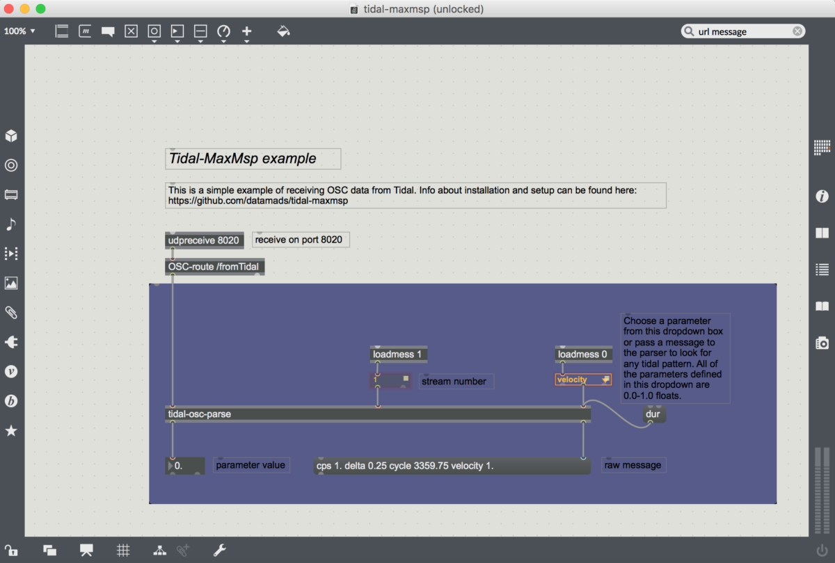
Once everything is installed, you should open up the tidal-maxmsp.maxproj. This is where you will receive the OSC data. Any of the standard tidal parameters are available as well as a few extra parameters defined in the MaxMspOsc module (see the dropdown on the right side of the patch which contains all of these custom parameters which are all float values of 0.0 to 1.0 for consistency’s sake).

At the top of the patch is a udpreceive object which is the network object that will receive the OSC data from tidal. It has one parameter defined, the port number, which is set to 8020 both here and in Tidal (you can change it another integer number as long as both Max MSP and Tidal are using the same port number).

Below it is an OSC-route object which looks for any OSC bundles with a url starting with /fromTidal and passes it on to the tidal-osc-parse abstraction.

If you double click the tidal-osc-parse abstraction you will see a small patch which has three inlets. The first is for the raw osc data from the OSC-route object. Inlet 2 receives the stream number (defined in Tidal) and inlet 3 takes the parameter name to look for. It breaks down the OSC message into pairs of parameters / values and looks for the one defined in inlet 3 and spits it out of it’s left outlet (and the raw message without any url at it’s right outlet).

Now, head back to Tidal and open up tidal-maxmsp-example.tidal. At the top of this file you’ll see an import statement for the Haskell module. Evaluate this line – if you don’t get an error, you most probably installed it correctly. Now evaluate max1 <- maxmspStream “127.0.0.1” 8020 1 and the last line to start sending OSC data.

If you head back to Max you should now see the values of the velocity pattern defined in Tidal now showing up in the float box in the bottom of the patch and all of the raw bundle in the message box.

That’s it!

Try connecting the float box to whatever Max MSP project you have, or if you want: Get more Tidal parameters by copying and pasting everything inside of the purple panel and changing the dropdown or message at the rightmost inlet of the tidal-osc-parse abstraction (and changing the tidal code accordingly).

Now, this is just a basic example which is not super precise in terms of timing. To get more precision we need to add time stamps/tags to make sure everything is played on time but this basic patch should get you started.

Elastic Tempo Flux

I just published a new tutorial video on how to achieve continuous, elastic tempo changes in TidalCycles.

The video covers techniques with two different functions: nudge and spaceOut.

nudge

You can use nudge to move the timing of events into the future. Here, we schedule each of the four cp samples with future times of 0, 0.7, 0.2, and 0.4 seconds, respectively:

d1 $ sound "cp*4" # nudge "0 0.7 0.2 0.4"

The above example isn’t very interesting. However, when you apply a sine function to nudge, you can make time appear to stretch in a smooth way:

d1 $ sound "cp*4" # nudge (slow 8 $ sine)

Different pattern densities, scaling, and sine speeds interact with each other to create different results:

d1 $ sound "cp*8" # nudge (range 0 2 $ slow 16 $ sine)

spaceOut

The spaceOut function lets you specify a list of cycle speed multipliers, and then plays the pattern exactly once at each speed:

d1 $ spaceOut [1, 0.5, 1.33, 0.1, 2] $ sound "cp*4 cp*2"

The above code will play the cp*4 cp*2 pattern at 1, then 0.5, 1.33, 0.1, and 2 times the normal cycle speed.

Where spaceOut gets a little more interesting is when you use Haskell’s list syntax to build longer lists of linear (or non-linear) values. Consider this spaceOut pattern that plays at speeds ranging from 1 to 3, incrementing by 0.1:

d1 $ spaceOut [1,1.1..3] $ sound "cp*4"

The above pattern has 30 different speeds (!) but with very little code.

You can achieve speed “oscillations” that resemble a triangle wave by adding two lists together with the ++ operator:

d1 $ spaceOut ([0.1,0.2..3] ++ [3,2.9..0.1]) $ sound "cp*4"

You can use many different Haskell features to build lists. Here is a different method that constructs lists of fractional values using map:

d1 $ spaceOut (map (1/) [1,1.5..10]) $ sound "cp*4"

How to Haskell – developing a Markov chain

One of my favorite things about Tidal is that it’s inside of Haskell, a well-developed full-blown programming language, so all sorts of tricks are available.  After some discussion on Slack I developed code for making Markov chains to use in Tidal, and here I’ll try to describe the process.

First – what’s a Markov chain? Basically it’s some kind of random sequence where each step depends only on the step immediately before it. A common way to express this is to imagine several possible “states” for each step, and then write a “transition matrix” which gives the odds of going from one state to another.

How should we represent all this in Tidal/Haskell?  We ultimately want to have the chain as a Pattern, but it’ll probably be easier to start out with an ordinary list, and then use the listToPat function to turn it into a Pattern.  Let’s number the states with integers, starting at zero.  Then the chain itself will be a list of integers.  The transition matrix is a list of lists of floating point numbers – we’ll use doubles. Then one way of writing things is to have a function that takes the transition matrix and a chain as arguments, and returns a new chain which is just the old one with one new element added. Here’s just the signature:

markovStep :: [[Double]] -> [Int] -> [Int]

Next let’s start the basic structure of what the function will have to do. Let’s call the transition matrix tp and the input chain xs. We need to look at the top element of the list to see what the “from” state is, and find that row of the transition matrix: tp!!(head xs). Next we need to generate a random number r (we’ll worry about how to actually do this later) and somehow use it to choose what the “to” state for the next step of the chain should be.

For example, if the row of the matrix were [0.20, 0.30, 0.50], this would mean 20% chance of transition to state zero, 30% chance to state one, and 50% chance to state two. So if our random number (between zero and one) were between 0 and 0.2, we’d pick state zero, between 0.2 and 0.5 state one, etc. This is easier to write if we take the cumulative sum of the row, and there’s a handy Haskell function we can use for that: scanl1 (+). That’ll turn the row into [0.20, 0.50, 1.00], and now when we have a random number we just need to find the index of the first element in the row larger than our random number. That’ll be the state the chain jumps to next.

There’s a handy Haskell function for finding things in lists too: findIndex. While it doesn’t quite work yet, we have most of our function:

markovStep tp xs = (findIndex (r <=) $ scanl1 (+) (tp!!(head xs))) : xs

(the : xs at the end adds the existing chain after the new element we just made)

One problem is that findIndex doesn’t actually return an Int. It returns a Maybe Int, because it might not find anything.  If our transition probabilities for each row add to one we’ll always be safe, but if we mess up or make a typo things might go wrong.  We have two options, (1) choose a safe default or (2) throw an exception and halt.  For the first option we could use fromMaybe 0 (to default to state zero), and for the second we’d use fromJust. Both require us to import the Data.Maybe module. Since I like to immediately know when I’ve made a math mistake and don’t mind if my performance grinds to a halt, I’m choosing the second option:

import Data.Maybe

markovStep tp xs = (fromJust $ findIndex (r <=) $ scanl1 (+) (tp!!(head xs))) : xs

The final thing to take care of is the random number. While it’s not quite the intended use, we can use the timeToRand function, which takes a rational number as an argument and hashes it to a pseudorandom result. We just have to make sure we get a different number for each step of the chain by using the length of the chain, and do type conversion as necessary:

import Data.Maybe

markovStep tp xs = (fromJust $ findIndex (r <=) $ scanl1 (+) (tp!!(head xs))) : xs 
  where r = timeToRand $ fromIntegral $ length xs

The last touch to make this a bit more usable is to wrap markovStep in a function that will repeat the step process to build a chain n numbers long from an initial state xi, flip it around so the most recent element is at the end, and turn the whole thing into a pattern with one number per cycle.

import Data.Maybe

markovStep :: [[Double]] -> [Int] -> [Int]
markovStep tp xs = (fromJust $ findIndex (r <=) $ scanl1 (+) (tp!!(head xs))) : xs 
  where r = timeToRand $ fromIntegral $ length xs
markovPat n xi tp = slow (fromIntegral n) $ listToPat 
  $ reverse $ (iterate (markovStep tp) [xi]) !! (n-1)

Now it’s ready to use in Tidal:

d1 
 $ fast 4 
 $ n (markovPat 64 0 [[0.3, 0.4, 0.3], [0.3, 0, 0.7], [0.7, 0.3, 0]])
 # s "arpy"

The chain states are always integers starting at zero, and that seems rather limiting.  But we can treat the chain as an index to some other array of our choice, which needn’t even be numerical:

d1
 $ fast 4
 $ n (fmap ([0,3,5]!!) $ markovPat 64 0 [[0.3, 0.4, 0.3], [0.3, 0, 0.7], [0.7, 0.3, 0]])
 # s "arpy"

d2
 $ fast 8
 $ s (fmap (["hc:2", "cr"]!!) $ markovPat 128 1 [[0.88, 0.12], [0.7, 0.3]])
 # cut 1

I’m sure there are still improvements we could make, but this is a pretty fun start!